HP OpenVMS Systems Documentation |
Guidelines for OpenVMS Cluster Configurations
9.5.2 AdvantagesConfiguration 3 offers the same individual component advantages as configuration 2, plus:
9.5.3 DisadvantagesConfiguration 3 has the following disadvantages:
9.5.4 Key Availability and Performance Strategies
Configuration 3 provides all the strategies of configuration 2 except
for physical separation of CIs. The major advantage over configuration
2 are the path-specific star coupler cabinets. They provide physical
isolation of the path A cables and the path A hub from the path B
cables and the path B hub.
The availability of a CI configuration can be further improved by physically separating shadow set members and their HSJ controllers. This significantly reduces the probability of a mechanical accident or other localized damage that could destroy both members of a shadow set. This configuration is shown in Figure 9-4. Figure 9-4 Redundant Components, Path-Separated Star Couplers, and Duplicate StorageWorks Cabinets (Configuration 4) 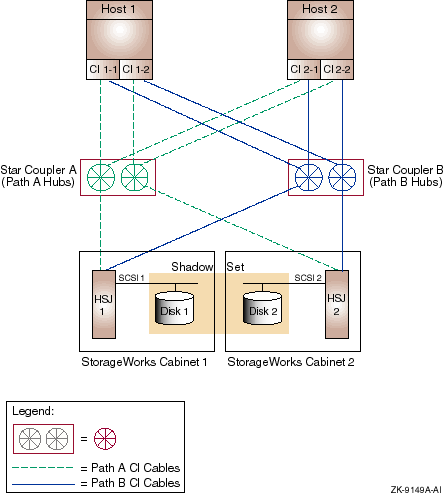
Configuration 4 is similar to configuration 3 except that the shadow set members and their HSJ controllers are mounted in separate StorageWorks cabinets that are located some distance apart. The StorageWorks cabinets, path-specific star coupler cabinets, and associated path cables should be separated as much as possible. For example, the StorageWorks cabinets and the star coupler cabinets could be installed on opposite sides of a computer room. The CI cables should be routed so that path A and path B cables follow different paths.
9.6.1 ComponentsThe CI OpenVMS Cluster configuration shown in Figure 9-4 has the following components:
9.6.2 AdvantagesConfiguration 4 offers most of the individual component advantages of configuration 3, plus:
9.6.3 DisadvantagesConfiguration 4 has the following disadvantages:
9.6.4 Key Availability and Performance Strategies
Configuration 4 (Figure 9-4) provides all of the strategies of
configuration 3. It also provides shadow set members that are in
physically separate StorageWorks cabinets.
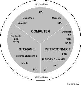
All four configurations illustrate how to obtain both availability and performance by:
An advanced technique, separating the CI path A and path B cables and associated hubs, is used in configuration 3 and configuration 4. This technique increases availability and maintains performance with no additional hardware. Configuration 4 provides even greater availability without compromising performance by physically separating shadow set members and their HSJ controllers. Using these configurations as a guide, you can select the techniques that are appropriate for your computing needs and adapt your environment as conditions change. The techniques illustrated in these configurations can be scaled for larger CI configurations.
Chapter 10
|
|||||||||||||||||||||||||||||||||||||||||||||||||||||||||||||||||||||||||||||||
| This Dimension | Grows by... |
|---|---|
| Systems | |
| CPU |
Implementing SMP within a system.
Adding systems to a cluster. Accommodating various processor sizes in a cluster. Adding a bigger system to a cluster. Migrating from VAX to Alpha systems. |
| Memory | Adding memory to a system. |
| I/O |
Adding interconnects and adapters to a system.
Adding MEMORY CHANNEL to a cluster to offload the I/O interconnect. |
| OpenVMS |
Tuning system parameters.
Moving to OpenVMS Alpha. |
| Adapter |
Adding storage adapters to a system.
Adding CI and DSSI adapters to a system. Adding LAN adapters to a system. |
| Storage | |
| Media |
Adding disks to a cluster.
Adding tapes and CD-ROMs to a cluster. |
| Volume shadowing |
Increasing availability by shadowing disks.
Shadowing disks across controllers. Shadowing disks across systems. |
| I/O |
Adding solid-state or DECram disks to a cluster.
Adding disks and controllers with caches to a cluster. Adding RAID disks to a cluster. |
| Controller and array |
Moving disks and tapes from systems to controllers.
Combining disks and tapes in arrays. Adding more controllers and arrays to a cluster. |
| Interconnect | |
| LAN |
Adding Ethernet and FDDI segments.
Upgrading from Ethernet to FDDI. Adding redundant segments and bridging segments. |
| CI, DSSI, Fibre Channel, SCSI, and MEMORY CHANNEL | Adding CI, DSSI, Fibre Channel, SCSI, and MEMORY CHANNEL interconnects to a cluster or adding redundant interconnects to a cluster. |
| I/O |
Adding faster interconnects for capacity.
Adding redundant interconnects for capacity and availability. |
| Distance |
Expanding a cluster inside a room or a building.
Expanding a cluster across a town or several buildings. Expanding a cluster between two sites (spanning 40 km). |
The ability to add to the components listed in Table 10-1 in any way
that you choose is an important feature that OpenVMS Clusters provide.
You can add hardware and software in a wide variety of combinations by
carefully following the suggestions and guidelines offered in this
chapter and in the products' documentation. When you choose to expand
your OpenVMS Cluster in a specific dimension, be aware of the
advantages and tradeoffs with regard to the other dimensions.
Table 10-2 describes strategies that promote OpenVMS Cluster
scalability. Understanding these scalability strategies can help you
maintain a higher level of performance and availability as your OpenVMS
Cluster grows.
10.2 Strategies for Configuring a Highly Scalable OpenVMS Cluster
The hardware that you choose and the way that you configure it has a
significant impact on the scalability of your OpenVMS Cluster. This
section presents strategies for designing an OpenVMS Cluster
configuration that promotes scalability.
10.2.1 Scalability Strategies
Table 10-2 lists strategies in order of importance that ensure scalability. This chapter contains many figures that show how these strategies are implemented.
| Strategy | Description |
|---|---|
| Capacity planning |
Running a system above 80% capacity (near performance saturation)
limits the amount of future growth possible.
Understand whether your business and applications will grow. Try to anticipate future requirements for processor, memory, and I/O. |
| Shared, direct access to all storage |
The ability to scale compute and I/O performance is heavily dependent
on whether all of the systems have shared, direct access to all storage.
The CI and DSSI OpenVMS Cluster illustrations that follow show many examples of shared, direct access to storage, with no MSCP overhead. Reference: For more information about MSCP overhead, see Section 10.8.1. |
| Limit node count to between 3 and 16 |
Smaller OpenVMS Clusters are simpler to manage and tune for performance
and require less OpenVMS Cluster communication overhead than do large
OpenVMS Clusters. You can limit node count by upgrading to a more
powerful processor and by taking advantage of OpenVMS SMP capability.
If your server is becoming a compute bottleneck because it is overloaded, consider whether your application can be split across nodes. If so, add a node; if not, add a processor (SMP). |
| Remove system bottlenecks | To maximize the capacity of any OpenVMS Cluster function, consider the hardware and software components required to complete the function. Any component that is a bottleneck may prevent other components from achieving their full potential. Identifying bottlenecks and reducing their effects increases the capacity of an OpenVMS Cluster. |
| Enable the MSCP server | The MSCP server enables you to add satellites to your OpenVMS Cluster so that all nodes can share access to all storage. In addition, the MSCP server provides failover for access to shared storage when an interconnect fails. |
| Reduce interdependencies and simplify configurations | An OpenVMS Cluster system with one system disk is completely dependent on that disk for the OpenVMS Cluster to continue. If the disk, the node serving the disk, or the interconnects between nodes fail, the entire OpenVMS Cluster system may fail. |
| Ensure sufficient serving resources | If a small disk server has to serve a large number disks to many satellites, the capacity of the entire OpenVMS Cluster is limited. Do not overload a server because it will become a bottleneck and will be unable to handle failover recovery effectively. |
| Configure resources and consumers close to each other | Place servers (resources) and satellites (consumers) close to each other. If you need to increase the number of nodes in your OpenVMS Cluster, consider dividing it. See Section 11.2.4 for more information. |
| Set adequate system parameters | If your OpenVMS Cluster is growing rapidly, important system parameters may be out of date. Run AUTOGEN, which automatically calculates significant system parameters and resizes page, swap, and dump files. |
Each CI star coupler can have up to 32 nodes attached; 16 can be
systems and the rest can be storage controllers and storage.
Figure 10-2, Figure 10-3, and Figure 10-4 show a progression from
a two-node CI OpenVMS Cluster to a seven-node CI OpenVMS Cluster.
10.3.1 Two-Node CI OpenVMS Cluster
In Figure 10-2, two nodes have shared, direct access to storage that includes a quorum disk. The VAX and Alpha systems each have their own system disks.
Figure 10-2 Two-Node CI OpenVMS Cluster
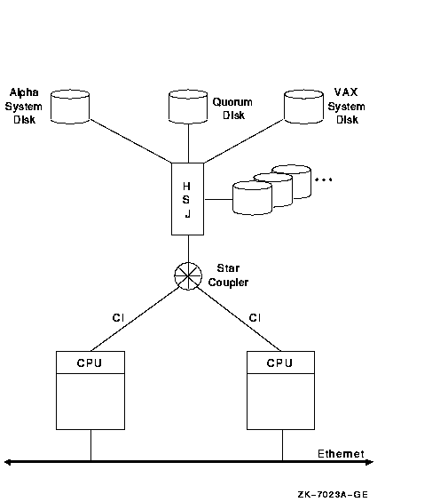
The advantages and disadvantages of the configuration shown in Figure 10-2 include:
An increased need for more storage or processing resources could lead
to an OpenVMS Cluster configuration like the one shown in Figure 10-3.
10.3.2 Three-Node CI OpenVMS Cluster
In Figure 10-3, three nodes are connected to two HSJ controllers by the CI interconnects. The critical system disk is dual ported and shadowed.
Figure 10-3 Three-Node CI OpenVMS Cluster
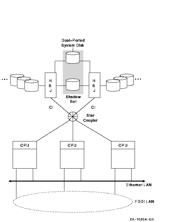
The advantages and disadvantages of the configuration shown in Figure 10-3 include:
If the I/O activity exceeds the capacity of the CI interconnect, this
could lead to an OpenVMS Cluster configuration like the one shown in
Figure 10-4.
10.3.3 Seven-Node CI OpenVMS Cluster
In Figure 10-4, seven nodes each have a direct connection to two star couplers and to all storage.
Figure 10-4 Seven-Node CI OpenVMS Cluster
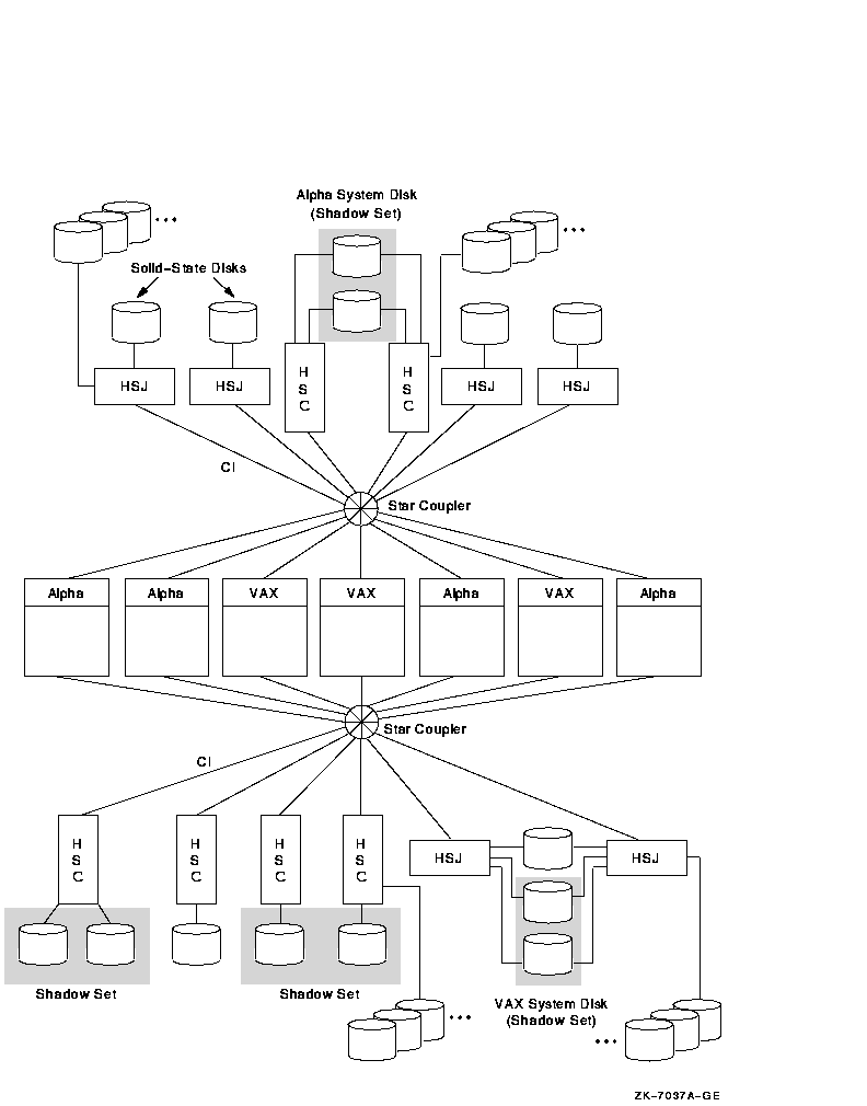
The advantages and disadvantages of the configuration shown in Figure 10-4 include:
The following guidelines can help you configure your CI OpenVMS Cluster:
Volume shadowing is intended to enhance availability, not performance. However, the following volume shadowing strategies enable you to utilize availability features while also maximizing I/O capacity. These examples show CI configurations, but they apply to DSSI and SCSI configurations, as well.
Figure 10-5 Volume Shadowing on a Single Controller
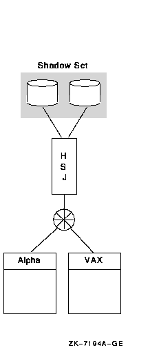
Figure 10-5 shows two nodes connected to an HSJ, with a two-member shadow set.
The disadvantage of this strategy is that the controller is a single point of failure. The configuration in Figure 10-6 shows examples of shadowing across controllers, which prevents one controller from being a single point of failure. Shadowing across HSJ and HSC controllers provides optimal scalability and availability within an OpenVMS Cluster system.
Figure 10-6 Volume Shadowing Across Controllers
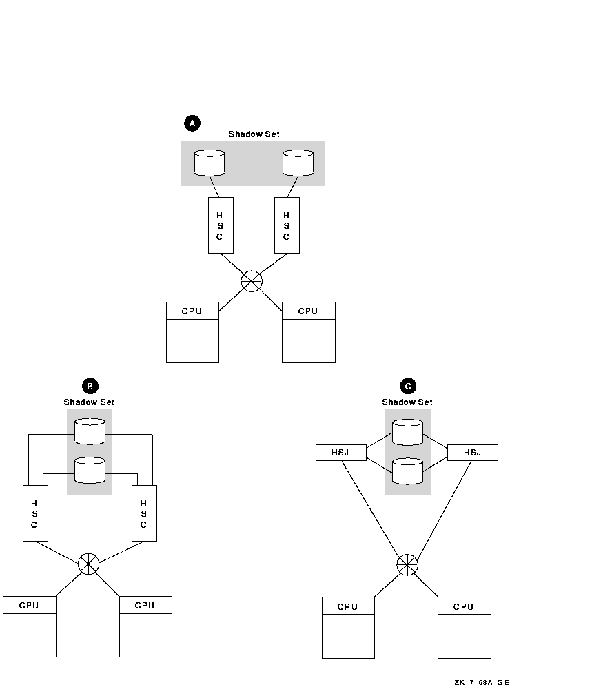
As Figure 10-6 shows, shadowing across controllers has three variations:
Figure 10-7 shows an example of shadowing across nodes.
Figure 10-7 Volume Shadowing Across Nodes
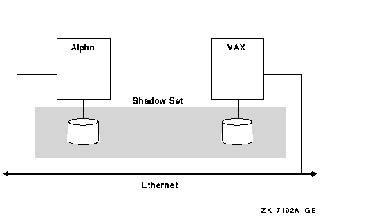
As Figure 10-7 shows, shadowing across nodes provides the advantage of flexibility in distance. However, it requires MSCP server overhead for write I/Os. In addition, the failure of one of the nodes and its subsequent return to the OpenVMS Cluster will cause a copy operation.
If you have multiple volumes, shadowing inside a controller and shadowing across controllers are more effective than shadowing across nodes.
Reference: See HP Volume Shadowing for OpenVMS for more information.
| Previous | Next | Contents | Index |